Power Take Off in Regenerative Auxiliary Power System
Modelling and Configuration
Many different factors and criteria should be considered in order to design an acceptable RAPS. To power the service vehicle's auxiliary devices from braking recovered energy, a regenerative braking system should be integrated into the vehicle powertrain. The connection of the RAPS to the vehicle powertrain, total system configuration, safety, weight, and size of components are the most important factors. As the first step, integration of the RAPS to the vehicle powertrain should be investigated in detail. It is vital that connection of the RAPS does not cause any major modification to the existing vehicle; otherwise, the initial cost of the total system and the safety concerns will reduce industry interest. The other important point is that the designed RAPS must be modular and easy-to-install in order to reduce installation time and costs. Additionally, this research is intended for use in any service vehicle with auxiliary devices, so RAPS components and especially their models should be generic, modular, and flexible for the creation of scalable powertrains and RAPS components models. Given these considerations, in this study, the RAPS components are designed with the different configurations of different powertrains in mind. By utilizing this method, RAPS components can be designed separately and added to an existing vehicle. In the first part of this chapter, the design configuration of the RAPS is discussed, and the two most possible categories for integration configurations are described. The modelling concepts of different RAPS components are explained in the last part.
System Configuration and Potential Energy Recovery
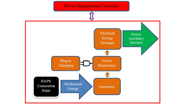
As illustrated in Figure 3.1, a RAPS consists of different electrical and mechanical parts. Input mechanical energy will be extracted from the vehicle's powertrain through the "RAPS Connection Point". There are different options for this connection point, and they will be explained in later sections. This extracted mechanical energy is in the form of torque and angular velocity. Based on the specifications and limitations of the generator, it is possible to change the range of the input angular velocity to the acceptable range of the generator.

Figure 3.1 Regenerative auxiliary power system (RAPS) configuration
The "Generator" will convert the mechanical energy into the electrical energy and produce electrical energy, in the form of current and voltage, to charge the "Electrical Energy Storages". The output energy of the generator will be sent to the "Electrical Energy Storages" through the "Power Electronics" module. The "Power Electronics" module controls the input energy flow to the "Electrical Energy Storages". The "Power Electronics" module function is to monitor the electrical energy flow and maintain the current and voltage in a form and range that is suitable for charging the "Electrical Energy Storages". As previously mentioned, the option for plug-in charging is considered for the proposed RAPS. The "Plug-in Charging" part will send the plug electrical energy to the "Electrical Energy Storages" through the "Power Electronics" module. The "Power Electronics" module has the ability to convert the plug-in AC electricity to the acceptable DC power by the "Electrical Energy Storage".
The "Electrical Energy Storages" stores the electrical energy and provides power to the vehicle's auxilary devices. The "Power Management Controller" will monitor the power demand, battery state of charge (SOC), vehicle status, and brake pedal signal, and based on these conditions, it will control the system's power flow. It should be noted that the one-way arrows in Figure 3.1 show the power flow in the RAPS, but the two-way arrow between the whole RAPS and the "Power Management Controller" is the flow of data and state conditions information.
System Integration to Powertrain
There are different parts in a vehicle powertrain that can be used to extract mechanical power for the generator. Possible configurations can be catagories in two main groups based on the amount of the demanded power; however, as explained in detail in the following sections, the limitation of the powertrain and connecting components are also very important in this classification. Two main groups of possible configurations are defined as:
Low Power Demand System (Serpentine Belt) Configuration
For service vehicles with power demands, it can be considered that the generator, which is mostly an alternator in this configuration, is connected to the engine's serpentine belt. The serpentine belt is a continuous belt used to power different devices, which are extracting their power directly from the engine. In this system, the serpentine belt connects the engine crankshaft to multiple devices including the alternator, water pump, air pump, air conditioning compressor, power steering pump, etc. In service vehicles, there is usually a space allocated to the attachment of another device, usually a compressor, to be powered by the serpentine belt. In the design of RAPS with low power demands, this space, as shown in Figure 3.2, can be used to install the extra generator. In addition, for service vehicles without this extra space, there is the option to utilize a higher output alternator instead of the Original Equipment Manufacturer (OEM) alternator.

Figure 3.2 Available space to install generator in the low power demand targeted vehicle "Ford Transit Connect Cargo XL-2010"
Figure 3.3 shows schematically the low power configuration and attachment of the generator to the engine. In this figure, the small arrows show the mechanical or electrical power flow and the big arrows emphasize the direction of the energy flow. The drawback of the low power demand configuration is that the maximum captured kinetic energy during braking is limited by the size of the generator-alternator. Thus, the regenerative energy is limited by the available space for the generator and the characteristics of the serpentine belt, especially its maximum tension capacity. This configuration is the main solution for vehicles, such as front wheel vehicles, with little space for adding the generator to the powertrain.

Figure 3.3 Low power demand systems (the serpentine belt) configuration
High Power Demand System (Power Take Off) Configurations
In service vehicles with high power demands, the generator can be driven by a power take off (PTO) module. In a vehicle, the engine produces power and transfers it to the wheels through the bell housing, transmission, drive shaft, differential and final axles. This condition can be better illustrated in a rear drive vehicle schematic as shown in Figure 3.4. In theory, it is possible to extract the mechanical power for the generator from 6 locations. However, PTO should allow RAPS to run directly from the engine when the vehicle is stopped. This option is possible if a PTO can be installed at a point between the engine and the transmission.

Figure 3.4 Possible power extraction (PTO Installation) points in the high power demand system configuration
In order to extract power at each of these points, a different PTO is needed. Generally, the required PTOs can be categorized into three main types;
- "Split Shaft PTO" : As shown in Figure 3.5, there are different designs and sizes for this kind of PTO. In Split Shaft PTOs, the input shaft runs two output shafts where one is a through shaft and the other is for power take off. Considering Figure 3.4, this type of PTO can be used in the following point:
Point 1: Shaft connecting engine to the bell housing
Point 2: Connecting the shaft of the bell housing of the transmission
Point 5: Driveline shaft (drive shaft)
Point 6: Any of the axles

Figure 3.5 "Split Shaft PTO"
It should be considered that in order to install the Split Shaft PTO, one of the power transferring shafts of the existing vehicle requires modification; also, for any of the considered points there should be enough space to install the PTO. Hence, from all the possible installation points for Split Shaft PTO, point 5 is the most acceptable one. This location, however, does not allow the generator run directly from the engine when the vehicle is stationary. Some Split Shaft PTO could be an option; however, it requires driver action which may make this solution generally undesirable.
- "Side Countershaft PTO": These types of PTOs are most common, and normally, they are just referred to as PTO- without any prefix. As shown in Figure 3.6, these PTOs will be installed to the output of the transmission. In most service vehicles or heavy-duty vehicles there is a place to install these PTOs. Considering Figure 3.4, this type of PTO can be used in:
Point 4: Transmission output to the drive shaft
However, installing a PTO for generator power extraction at Point 4 has the same setback as Point 5 and may not be desirable.

Figure 3.6 "Side Countershaft PTO"
- "Transmission Aperture PTO": In most heavy-duty vehicles, especially service vehicles, the option for mechanical powering of extra devices has been allocated. In these cases, as shown in Figure 3.7, the vehicle transmission has a special place for installing a "Transmission Aperture PTO" to power up other devices. Considering Figure 3.4, this type of PTO can be used in:
Point 3: Transmission Aperture

Figure 3.7 "Transmission Aperture PTO"
There are different scenarios that should be considered for all configurations:
I) Braking: It is expected that RAPS employs the waste energy during braking and maximizes the use of regenerative braking energy. The system will be considered to be in the regenerative braking phase if all the following conditions are met:
1. The vehicle is braking (braking signal is sent to the controller)
2. The vehicle speed is higher than a threshold (higher than 16 km/h based on suggestion)
3. The EES is not full (battery SOC level is lower than 100%)
For a low power demand system (serpentine belt) configuration during braking, in an automatic transmission, the torque converter still gets braking powers from the drive wheels to pass on the serpentine belt. However, in manual transmissions (or automatic transmissions at very low vehicle speeds) during braking, the clutch will disconnect the engine-belt from the transmission (or the torque converter does not pass the remaining braking energy.); thus, regenerative braking energy is just part of the kinematic energy in the crankshaft and moving inertia of the engine.
For the high power demand system (PTO) configuration, segments of the drive wheel braking powers, kinetic energy in the crankshaft, and moving inertia of engine during braking can be converted into the regenerative braking power. For this configuration, in manual transmissions during braking, the clutch will disconnect the engine from the transmission and other parts of the driveline. Therefore, if point 1 is considered as the RAPS connection point to vehicle drivetrain, regenerative braking energy will be just part of the kinetic energy in the crankshaft and moving inertia of the engine. Conversely, if any of points 3,4,5 and 6 is considered as the connection point, regenerative braking energy will be limited to part of the braking power from the drive wheels. It should be noted that in most vehicles targeted for high power demand configuration, the bell housing (clutch/torque-converter) is a part of transmission package since connection point 2 will have the same conditions as connection point 3 in most cases.
For the high power demand system (PTO) configuration in automatic transmissions, the bell housing will not disconnect any part of the vehicle powertrain during braking; thus, regenerative braking energy can be obtained from the drive wheel braking powers, kinetic energy in the crankshaft, and moving inertia of engine altogether. Additionally during very low vehicle speeds, the second condition of the regenerative braking phase is not satisfied; therefore, there will be no regenerative braking when that bell housing disconnects the engine from the other parts of vehicle powertrain.
II) Vehicle Movement: If regenerative braking energy is not sufficient to charge the batteries, the power management controller charges the batteries directly from the engine during peak engine performance. In this scenario, since the moving power is transferred from the engine all the way to the drive wheels, RAPS can extract the power in all of the aforementioned possible configurations.
III) Vehicle Stops: The RAPS target is to prevent the vehicle from idling; hence, while the vehicle is stopped, the engine ought not be active. During long stops, the auxiliary devices power consumption decreases the battery SOC to a critical level. In this condition, the system should allow a generator to be run directly from the engine when the vehicle is stopped. A serpentine belt configuration will work without any limitations in this scenario. For the PTO configurations, the power extraction point should be anywhere between the engine and the vehicle transmission, or the option of a PTO with a disconnecting clutch and driver action should be considered.
Given all of these scenarios, the "Transmission Aperture PTO" is the ideal and the most cost effective solution for the realization of the RAPS in high power demand service vehicles.
Components Modelling
As the system model will be used for the optimization process, the components models should be generic, modular and flexible. The components models need to be scalable so that the optimization method can determine their optimal sizes.
There are two modelling approaches that can be used:
a) Forward-looking: As shown in Figure 3.8, modelling and simulation starts from the driver's points of view. The driver's demanded power is sent to the powertrain components, and the resulting power that is available from the powertrain is fed to the final drive and wheels. This type of modelling is more realistic compared to the backward looking models.

Figure 3.8 General forward-looking vehicle model
b) Backward Looking: In this approach, the required power is determined based on the known drive cycle data. Illustrated in Figure 3.9, this power demand is then calculated and transferred through the powertrain components to the engine or another main power source. Through this process and using the components' efficiencies, the power needed in each component is calculated. In this approach, the detailed dynamics of the components and the vehicle system is not considered; however, this will crate less complicated models compared to the forward-looking models, which require solving differential equations.

Figure 3-9: General backward looking vehicle model
Based on the fact that in this study, only the overall power consumption of the vehicle is of interest, the effects of vehicle dynamics due to the suspension can be safely ignored even though the model is not as realistic as the forward-looking model. The backward-looking approach modeling is chosen for this work to fulfill the purpose of optimization. Simultaneously, the developed vehicle model formulation is suitable for the power consumption objectives. The total system model consists of powertrain components (engine, bell housing, transmission, differential) and RAPS components (batteries, power electronic, generator, auxiliary load). The goal of this research is to design and optimize a suitable regenerative braking system, which can be added to a service vehicle’s powertrain. As previously mentioned, the modifications to the vehicle powertrain should be kept to a minimum to make the changes affordable for the industrial purposes. Thus, there should not be any change to the configuration of the mechanical components of the vehicle. The powertrain components are modeled using the scalable backward-looking approach proposed by the Guzzella and Rizzoni [43]. In this approach, the actual consumed power of a component is calculated by multiplying the required component torque and component current velocity given the component’s efficiencies.
General Vehicle Model
In order to fulfill the need for a simple model for the backward-looking modeling approach, a simple vehicle body model is considered. This model only utilizes the drive torque, rolling resistance, and the resistive aerodynamic forces. The vehicle body model receives the demanded longitudinal velocity of vehicle (𝑉𝐷𝑒𝑠) and demanded longitudinal acceleration of vehicle (𝐴𝐷𝑒𝑠) as the input data. Based on these, the model calculates the torque (𝑇𝑊ℎ𝑒𝑒𝑙) and angular velocity (𝜔𝑊ℎ𝑒𝑒𝑙) at the wheels (or axles) as follows:
Wwheel = (Vdes)/(Reff)
Twheel = (Ftotal)x(Reff)
in which:
𝐹𝑇𝑜𝑡𝑎𝑙 = 𝐹𝐷𝑟𝑖𝑣𝑒 + 𝐹𝐷𝑟𝑎𝑔 + 𝐹𝑅𝑅
and
𝐹𝐷𝑟𝑖𝑣𝑒 = 𝑀𝑇𝑜𝑡𝑎𝑙 𝐴𝐷𝑒𝑠
Wwheel = (Vdes)/(Reff)
Twheel = (Ftotal)x(Reff)
in which:
𝐹𝑇𝑜𝑡𝑎𝑙 = 𝐹𝐷𝑟𝑖𝑣𝑒 + 𝐹𝐷𝑟𝑎𝑔 + 𝐹𝑅𝑅 |
and
𝐹𝐷𝑟𝑖𝑣𝑒 = 𝑀𝑇𝑜𝑡𝑎𝑙 𝐴𝐷𝑒𝑠 |
Fdrag = (1/2)(Cd)(𝜌)(Vdes)^2(A)
𝐹𝑅𝑅 = 𝐶𝑅𝑅 𝑀𝑇𝑜𝑡𝑎𝑙 𝑔 cos 𝛼

where 𝐹𝑇𝑜𝑡𝑎𝑙 , 𝐹𝐷𝑟𝑖𝑣𝑒 , 𝐹𝐷𝑟𝑎𝑔 , and 𝐹𝑅𝑅 represents total vehicle longitudinal force, drive force, total aerodynamics drag force, and total tire rolling resistance force, respectively. 𝐶𝐷 is the drag coefficient, 𝜌 is the air density, 𝐴 is the frontal area of vehicle, 𝐶𝑅𝑅 is the rolling resistance of the tire, 𝑔 is the gravitational acceleration, 𝛼 is the road grade angle in radian, 𝑅𝐸𝑓𝑓 is the effective tire radius, and 𝑀𝑇𝑜𝑡𝑎𝑙 is total vehicle mass, which is considered to be:
𝑀𝑇𝑜𝑡𝑎𝑙 = 𝑀𝑉𝑒ℎ + 𝑀𝐸𝐸𝑆 + 𝑀𝐶𝑎𝑟𝑔𝑜
where 𝑀𝑉𝑒ℎ is the vehicle mass before installing the EES packs or loading the cargo, 𝑀𝐶𝑎𝑟𝑔𝑜 is the cargo weight of the vehicle and 𝑀𝐸𝐸𝑆 is the mass of the electrical energy storage (EES) and other electrical parts. The total drive power demand (𝑃𝐷𝑟𝑖𝑣𝑒), the power needed to move the vehicle, is equal to:
𝑃𝐷𝑟𝑖𝑣𝑒 = 𝜔𝑊ℎ𝑒𝑒𝑙 𝑇𝑊ℎ𝑒𝑒𝑙 + 𝑃𝐿𝑜𝑠𝑡
in which 𝑃𝐿𝑜𝑠𝑡 is the lost power in the powertrain system.
Final Drive (Differential)
The demand torque and angular velocity at the wheels (or axles) are the inputs for the final drive. After applying the final drive ratio (𝑁𝐹), the demand torque (𝑇𝐷𝐿) and angular velocity (𝜔𝐷𝐿) at the driveline are calculated as:
𝜔𝐷𝐿 = 𝑁𝐹 𝜔 𝑊ℎ𝑒𝑒𝑙
Tdl = (Twheel)/(Nnr*nf)
where 𝜂𝐹 is the final drive efficiency.
PTO
The PTO consists of a set of gears that transfer the extracted mechanical power from the powertrain to the generator in the high power demand configuration. In order to keep the model as simple as possible, the PTO is modeled by a gear ratio (𝑁𝑃𝑇𝑂) and an efficiency factor (𝜂𝑃𝑇𝑂). The modeling formula for the PTO defines its output torque (𝑇𝑃𝑇𝑂−𝑂𝑢𝑡), which is equal to the generator torque in the high power demand configuration, and its output angular velocities (𝜔𝑃𝑇𝑂−𝑂𝑢𝑡) as:
𝐹𝑅𝑅 = 𝐶𝑅𝑅 𝑀𝑇𝑜𝑡𝑎𝑙 𝑔 cos 𝛼 |
![]()
𝑀𝑇𝑜𝑡𝑎𝑙 = 𝑀𝑉𝑒ℎ + 𝑀𝐸𝐸𝑆 + 𝑀𝐶𝑎𝑟𝑔𝑜 |
where 𝑀𝑉𝑒ℎ is the vehicle mass before installing the EES packs or loading the cargo, 𝑀𝐶𝑎𝑟𝑔𝑜 is the cargo weight of the vehicle and 𝑀𝐸𝐸𝑆 is the mass of the electrical energy storage (EES) and other electrical parts. The total drive power demand (𝑃𝐷𝑟𝑖𝑣𝑒), the power needed to move the vehicle, is equal to:
𝑃𝐷𝑟𝑖𝑣𝑒 = 𝜔𝑊ℎ𝑒𝑒𝑙 𝑇𝑊ℎ𝑒𝑒𝑙 + 𝑃𝐿𝑜𝑠𝑡 |
in which 𝑃𝐿𝑜𝑠𝑡 is the lost power in the powertrain system.
Final Drive (Differential)
The demand torque and angular velocity at the wheels (or axles) are the inputs for the final drive. After applying the final drive ratio (𝑁𝐹), the demand torque (𝑇𝐷𝐿) and angular velocity (𝜔𝐷𝐿) at the driveline are calculated as:
𝜔𝐷𝐿 = 𝑁𝐹 𝜔 𝑊ℎ𝑒𝑒𝑙 | |
Tdl = (Twheel)/(Nnr*nf) |
PTO
| Tpto-out = (Tpto-in)/(Npto)npto*Cact-pto | |
𝜔𝑃𝑇𝑂−𝑂𝑢𝑡 = 𝑁𝑃𝑇𝑂 𝜔𝑃𝑇𝑂−𝐼𝑛 |
in which 𝐶𝐴𝑐𝑡−𝑃𝑇𝑂 is the PTO activation control signal provided by the power management controller. In a high power demand configuration, the PTO is responsible for extracting the energy from the powertrain for the generator. This power extraction occurs in two general cases: i) Battery pack SOC decreases to a critical level where the power management controller decides to charge the battery pack (during the vehicle’s movement or stop); and ii) regenerative braking. In either of the two general cases, the PTO’s activation control signal will be one (active); otherwise this value will be zero (not active).
The power management controller, in general, controls the flow of power by monitoring the auxiliary power demand, battery state of the charge, vehicle status, brake pedal signal, and amount of power produced by the generator. Power management is considered as a higher level control algorithm that monitors the power flow between the vehicle powertrain, generator, and ESS as shown in Figure 3-10. The controller makes sure that the generator produces the maximum amount of power during regenerative braking to maximize the RAPS efficiency. In addition, the controller charges the batteries directly from the engine, during the peak engine performance, when the state of the charge is lower than a critical value.

Figure 3-10: Power management controller input/output signals
In order to determine when to charge the batteries with the direct power from the engine, the controller considers the following criteria:
1. Once the SOC drops below the “High-level battery SOC threshold”, the engine will be used to charge the battery packs if it is working at high efficiency (30% or higher);
2. Once the SOC drops below the critical value or “Low-level battery SOC threshold”, the engine will be used to charge the battery packs under any condition, even low efficiency or idling, to prevent battery packs from any damage and life cycle reduction;
3. During braking conditions, there will certainly be no direct charging from the engine.
In order to make the system model as simple as possible, the controller utilizes a rule-based strategy that is adequate for control purposes in the design optimization of the proposed RAPS. The low and high-level battery SOC thresholds are defined in the optimization process, and will be further explained in Chapter 4.
Transmission (Gearbox)
The demand torque and angular velocity at the transmission output shaft (driveline) are the inputs to transmission model. After applying the transmission ratio (𝑁𝑇), the demand torque (𝑇𝑇 ) and angular velocity (𝜔𝑇) at the transmission are calculated as transmission model outputs:
𝜔𝑇 = 𝑁𝑇 𝜔𝐷𝐿
Tt = (Tdl)/(Nt*nt)
in which 𝜂𝑇 represents the transmission efficiency. The values of the transmission ratio are calculated using a look-up table indexed by the vehicle’s longitudinal speed. It should be mentioned that the connection between the transmission and engine is provided by the bell housing (clutch / torque-convertor). Due to the fact that a simple component modeling approach is selected for this study, the effects of the bell housing part are considered in the transmission efficiency.
Generator
The output electrical power of the generator (𝑃𝐺), in the form of output current (𝐼𝐺) and output voltage (𝑉𝐺) is calculated as:
𝑃𝐺 = 𝐼𝐺𝑉𝐺 = 𝜂𝐺 𝑇𝐺𝜔𝐺
 where the 𝑇𝐺 and 𝜔𝐺 are the input torque and angular velocity to the generator, and 𝜂𝐺 is the generator efficiency from the lookup tables indexed by the input torque and angular velocity to the generator. In the low power demand configuration, the generator is connected to the engine through the serpentine belt. During regenerative braking, the bell housing transfers braking powers from the transmission to the serpentine belt. In this case:
Tg = (areg*Tt)/(Ng)
𝜔𝐺 = 𝑁𝐺𝜔𝑇
 in which 𝛼𝑅𝑒𝑔 is the regenerative braking coefficient and 𝑁𝐺 is the generator ratio due to serpentine belt pulleys. During braking conditions (due to safety, general limitations of adding regenerative braking, system efficiency, and size limitation of the generator), conventional mechanical brakes still work. Therefore, by adding regenerative braking to the vehicle, just a percentage of the braking torque energy can be captured by the generator. The regenerative braking coefficient (𝛼𝑅𝑒𝑔) represents this percentage. On the other hand, during vehicle movement or vehicle stop scenarios, the generator demanded torque, which is determined by the controller as it charges the battery in a critical level SOC, will be provided by the engine. In these cases:
Tg = (Te_charge)/(Ng)
𝜔𝐺 = 𝑁𝐺𝜔𝐸
where 𝑇𝐸_𝐶ℎ𝑎𝑟𝑔𝑒 is the engine demand torque for direct battery charging conditions (when the generator is run by the engine instead of regenerative breaking energy). In these scenarios, the engine demanded torque for direct charging (𝑇𝐸_𝐶ℎ𝑎𝑟𝑔𝑒 ) will be added to the transmission demanded torque (𝑇𝑇) and the required torque to overcome the resistance forces at the engine (𝑇𝑅) in order to determine the total demand torque from the engine (𝑇𝐸):
𝑇𝐸 = 𝑇𝑅 + 𝑇𝑇 + 𝑇𝐸𝐶ℎ𝑎𝑟𝑔𝑒
𝜔𝐸 = 𝜔𝑇
Based on the fuel consumption rate during idling, the engine idling torque is estimated and this value is considered to be the needed torque to overcome the engine resistance forces (𝑇𝑅).

In the high power demand configuration, a generator is connected to the PTO. Therefore, generator torque and angular velocity are equal to the output torque of the PTO (𝑇𝑃𝑇𝑂−𝑂𝑢𝑡) and output angular velocities of the PTO (𝜔𝑃𝑇𝑂−𝑂𝑢𝑡), respectively. When considering the “Transmission Aperture” PTO configuration in the regenerative braking phase, the generator torque and angular velocity are determined as:
𝜔𝐺 = 𝑁𝑃𝑇𝑂𝜔𝑇
During vehicle movement or vehicle stop scenarios, if the battery SOC decreases to the critical level, the generator will be powered directly by the engine (direct battery charging). In these scenarios, the generator torque is calculated as:
In order to make the system model as simple as possible, the controller utilizes a rule-based strategy that is adequate for control purposes in the design optimization of the proposed RAPS. The low and high-level battery SOC thresholds are defined in the optimization process, and will be further explained in Chapter 4.
Transmission (Gearbox)
The demand torque and angular velocity at the transmission output shaft (driveline) are the inputs to transmission model. After applying the transmission ratio (𝑁𝑇), the demand torque (𝑇𝑇 ) and angular velocity (𝜔𝑇) at the transmission are calculated as transmission model outputs:
𝜔𝑇 = 𝑁𝑇 𝜔𝐷𝐿 | |
Tt = (Tdl)/(Nt*nt) |
![]() in which 𝜂𝑇 represents the transmission efficiency. The values of the transmission ratio are calculated using a look-up table indexed by the vehicle’s longitudinal speed. It should be mentioned that the connection between the transmission and engine is provided by the bell housing (clutch / torque-convertor). Due to the fact that a simple component modeling approach is selected for this study, the effects of the bell housing part are considered in the transmission efficiency.
in which 𝜂𝑇 represents the transmission efficiency. The values of the transmission ratio are calculated using a look-up table indexed by the vehicle’s longitudinal speed. It should be mentioned that the connection between the transmission and engine is provided by the bell housing (clutch / torque-convertor). Due to the fact that a simple component modeling approach is selected for this study, the effects of the bell housing part are considered in the transmission efficiency.
Generator
The output electrical power of the generator (𝑃𝐺), in the form of output current (𝐼𝐺) and output voltage (𝑉𝐺) is calculated as:
𝑃𝐺 = 𝐼𝐺𝑉𝐺 = 𝜂𝐺 𝑇𝐺𝜔𝐺 |
![]() where the 𝑇𝐺 and 𝜔𝐺 are the input torque and angular velocity to the generator, and 𝜂𝐺 is the generator efficiency from the lookup tables indexed by the input torque and angular velocity to the generator. In the low power demand configuration, the generator is connected to the engine through the serpentine belt. During regenerative braking, the bell housing transfers braking powers from the transmission to the serpentine belt. In this case:
where the 𝑇𝐺 and 𝜔𝐺 are the input torque and angular velocity to the generator, and 𝜂𝐺 is the generator efficiency from the lookup tables indexed by the input torque and angular velocity to the generator. In the low power demand configuration, the generator is connected to the engine through the serpentine belt. During regenerative braking, the bell housing transfers braking powers from the transmission to the serpentine belt. In this case:
Tg = (areg*Tt)/(Ng)
𝜔𝐺 = 𝑁𝐺𝜔𝑇 |
![]() in which 𝛼𝑅𝑒𝑔 is the regenerative braking coefficient and 𝑁𝐺 is the generator ratio due to serpentine belt pulleys. During braking conditions (due to safety, general limitations of adding regenerative braking, system efficiency, and size limitation of the generator), conventional mechanical brakes still work. Therefore, by adding regenerative braking to the vehicle, just a percentage of the braking torque energy can be captured by the generator. The regenerative braking coefficient (𝛼𝑅𝑒𝑔) represents this percentage. On the other hand, during vehicle movement or vehicle stop scenarios, the generator demanded torque, which is determined by the controller as it charges the battery in a critical level SOC, will be provided by the engine. In these cases:
in which 𝛼𝑅𝑒𝑔 is the regenerative braking coefficient and 𝑁𝐺 is the generator ratio due to serpentine belt pulleys. During braking conditions (due to safety, general limitations of adding regenerative braking, system efficiency, and size limitation of the generator), conventional mechanical brakes still work. Therefore, by adding regenerative braking to the vehicle, just a percentage of the braking torque energy can be captured by the generator. The regenerative braking coefficient (𝛼𝑅𝑒𝑔) represents this percentage. On the other hand, during vehicle movement or vehicle stop scenarios, the generator demanded torque, which is determined by the controller as it charges the battery in a critical level SOC, will be provided by the engine. In these cases:
Tg = (Te_charge)/(Ng)
𝜔𝐺 = 𝑁𝐺𝜔𝐸 |
where 𝑇𝐸_𝐶ℎ𝑎𝑟𝑔𝑒 is the engine demand torque for direct battery charging conditions (when the generator is run by the engine instead of regenerative breaking energy). In these scenarios, the engine demanded torque for direct charging (𝑇𝐸_𝐶ℎ𝑎𝑟𝑔𝑒 ) will be added to the transmission demanded torque (𝑇𝑇) and the required torque to overcome the resistance forces at the engine (𝑇𝑅) in order to determine the total demand torque from the engine (𝑇𝐸):
𝑇𝐸 = 𝑇𝑅 + 𝑇𝑇 + 𝑇𝐸𝐶ℎ𝑎𝑟𝑔𝑒 | |
𝜔𝐸 = 𝜔𝑇 |
Based on the fuel consumption rate during idling, the engine idling torque is estimated and this value is considered to be the needed torque to overcome the engine resistance forces (𝑇𝑅).
![]()
𝜔𝐺 = 𝑁𝑃𝑇𝑂𝜔𝑇 |
During vehicle movement or vehicle stop scenarios, if the battery SOC decreases to the critical level, the generator will be powered directly by the engine (direct battery charging). In these scenarios, the generator torque is calculated as:
Tg = (areg*Tt)/(Npto)npto*Cact-pto | |
𝜔𝐺 = 𝑁𝑃𝑇𝑂 𝜔𝐸 |
![]()
Similarly, in the low power demand configuration, for the direct battery charging condition in the “Transmission Aperture”, the PTO configuration equations (3-20) and (3-21) are valid.
Engine
The engine model should be scalable so that the developed model can be easily modified for different vehicles. Similar to the model used in [43], the applied engine model in this study has the scalability and composability features. Using a scalable model, the vehicle components that belong to the same class (for example ICEs) can be modeled using the same basic model. The important factor is that the model should be independent from the component size and can be scaled based on a simple scalar variable such as displacement or power rating. The composability feature is concerned that the system components’ model can easily compose the other related parts.
Storing, converting, and transferring the energy in a vehicle is concerned with three domains: chemical, mechanical, and electrical. In each energy domain, power is equal to the product of flow variable and effort variable. In the powertrain analysis, angular velocity and torque are the flow and effort variables, respectively [44]. The Willan’s line modeling approach, which is proposed by Rizzoni et al. [49], normalizes the flow and effort variables to create a model that is independent of scaling. The Willan’s line concept for a generic energy converter, ICE in this case, is shown in Figure 3-11.

This approach relates the available input energy for conversion (𝑾𝑰𝒏), to the actual useful output energy of the converter (𝑾𝑶𝒖𝒕) as follows:
𝑊𝑂𝑢𝑡 = 𝑒𝑊𝐼𝑛 − 𝑊𝐿𝑜𝑠𝑠 |
![]()
![]()
![]()
n = (Wout/(Win) = (eWin-Wloss)/(Win) = e- (Wloss)/(Win)
It is obvious that “the actual conversion efficiency is a function of the operating conditions of the converter” [43], and this efficiency will be maximized when the ratio of energy losses to input energy is minimized. In a general ICE, the following equation is valid [43]:
𝜔𝐸 𝑇𝐸 = 𝜂𝐸 𝑃𝐹𝑢𝑒𝑙 = 𝜂𝐸 𝑚̇ 𝐹𝐻𝐿 |
in which 𝑃𝐹𝑢𝑒𝑙 represents the enthalpy flow associated with the fuel mass flow, 𝜂𝐸 is the engine efficiency, 𝑚̇ 𝐹 is the fuel mass flow, and 𝐻𝐿 is fuel’s lower heating value. In equation (3-28), engine efficiency is defined based on dimensional variables that depend on the engine’s size. In order to develop a scalable engine model, which is independent of the power rating or displacement and can be used for size optimization, Willan’s line scalable engine model is utilized to calculate the engine efficiency. As proposed by Guzzella and Rizzoni [43], [44], using normalizations based on the ICE’s characteristics, this dependency can be avoided. In this approach, the scalable model of the engine is developed based on three parameters:
![]()
![]()
![]()
pme = (N𝜋)/(Ved)*Te
pmf = (N𝜋Hlmf)/(Ved*we)
Vmp = (S*We)/(𝜋)
![]()
ne = (Pme)/(nmf)
Based on the concepts of thermodynamic efficiency and internal losses during the engine cycle, the mean effective pressure (𝑝𝑀𝐸) is calculated as:
𝑝𝑀𝐸 = 𝑒𝐸 𝑝𝑀𝐹 − 𝑝𝐿 |
in which 𝑒𝐸 is the thermodynamic properties of the engine related to the mean effective pressure, and 𝑝𝐿 is the engine losses where:
𝑝𝐿 = 𝑝𝐿𝐺 + 𝑝𝐿𝐹 |
![]()
𝑝 = 𝑘 (𝑘 + 𝑘 (𝑆𝜔 )2) 𝛱 𝑘4 𝐿𝐹 1 2 3 𝐸 𝑚𝑎𝑥 √ 𝐵 |
where 𝐵 is the engine cylinder bore, 𝛱𝑚𝑎𝑥 is the maximum boost pressure, and 𝑘 parameters are experimental parameters. Using equations (3-32), (3-33), (3-34), and (3-35), 𝜂𝐸 is determined. Also, the fuel consumption can be calculated for a given engine output torque and speed.
In the model developed in this study, the engine model receives the demand torque and angular velocity as the inputs. The engine efficiency (𝜂𝐸) is calculated based on the aforementioned method, and sent to the controller as the engine model output. Also, based on equation (3-28) and 𝜂𝐸 value, the required fuel (fuel mass flow of 𝑚̇ 𝐹) can be calculated as the second output of the engine model as follows:
𝜔𝐸𝑇𝐸 𝑚̇ 𝐹 = 𝐻 𝜂 𝐿 𝐸 |
Electrical Energy Storage Systems (Batteries)
If considering the electric circuit-based modeling approach, there are different models developed for the batteries. A comparison among seven common circuit-based models is presented in [46]. It is concluded that “Dual Polarization (DP)” and “Thevenin” models perform best since the impact of the battery relaxation effect is considered for their modeling. As illustrated in Figure 3-12, both Dual Polarization and Thevenin models are based on a simpler model known as internal resistance model or “Rint”.

The “Thevenin” model is created by adding an RC network to the “Rint” model and “Dual Polarization” is created by adding an RC network to the “Thevenin” model. Each RC network consists of a resistor (R) and a capacitor (C). In Figure 3-12, R1, R2, and R3 represent the effect of the series resistance, long time transient resistance, and short time transient resistance of the battery, respectively. In addition, V1, V2, and V3 represent the terminal voltage, long time transient voltage, and short time transient voltage of the battery, respectively. Finally, C1 and C2 represent the long time transient capacitance and short time transient capacitance of the battery, respectively. It should be considered that in the “Thevenin” model, the set of C1, V2, and R2 are just considered as the representatives of the transient time changes. However, in the “Dual Polarization” model the set of C2, V3, and R3 is added to represent the short time transient changes and the set of C1, V2, and R2 represent the long time transient changes.
It is possible to add more RC networks to the “Rint” model; however, adding more RC networks increases the complexity and computational cost of the model without improving model accuracy. On the other hand, based on experiments performed by [46] and [50], adding more than two RC networks decreases the performance of some aspects of the model. According to [46], the “Dual Polarization” model performs best among common electric circuit-based battery models followed by the “Thevenin” model. However, both of these models are created based on the “Rint” model, and considering experimental results [46], [49], the performance of the “Rint” model is close to the performance of the “Dual Polarization” and the “Thevenin” models, especially considering the interests and conditions of this study. From [46], the maximum error in the Hybrid Pulse Power Characterization (HPPC) tests [51] for a battery cell with nominal voltage of 3.2 V, is less than 40 [mV](1.25%) for the “Dual Polarization” and the “Thevenin” models, and less than 180 [mV] (%5) for the “Rint” model; however, the mean error for all three models is less than 10 [mV] (0.3%).
The “Thevenin” and “Rint” models are compared in [55]. The comparison shows that in a city drive cycle such as the UDDS, which is the main part of service vehicles working drive cycle, the difference between two battery models is small. This is similar to the results of [52], where it is considered that the “Rint” model has a performance error around 5% compared to “Thevenin” model. Therefore, although the battery’s dynamic voltage performance is ignored in the “Rint” model, in the working condition of service vehicles, the performance of the “Dual Polarization”, the “Thevenin”, and the “Rint” models are close. Due to this fact and considering that one of the main objectives of this research is to develop a method that can be easily used to design RAPS for different service vehicles, the “Rint” model is selected for battery modeling. This model will not increase the computational cost. More importantly, it does not need different battery parameters, such as C1, C2, V2, V3, R3, and R3, which are generally not provided by the battery manufacturer. There is a need for performing characterization tests such as HPPC [51] to identify these parameters. This process is not of interest in RAPS design for different service vehicles and the fleet companies.
Rint Battery Model
𝑃𝐵_Desired = 𝑅𝐼𝑛𝐼2 + 𝑉𝐵_𝑂𝐶 𝐼𝐵 𝐵 |
in which 𝑅𝐼𝑛 , 𝐼𝐵, and 𝑉𝐵_𝑂𝐶 represent the internal resistance, current, and the open circuit voltage of the battery, respectively. It is assumed that when the battery is being charged, the current and the subsequent desired change in the battery power (𝑃𝐵_Desired) are both positive. Conversely, when the battery is being discharged, the current and the desired change in the battery power (𝑃𝐵_Desired) are both negative. It should be mentioned that the first term of equation (3-37), 𝑅𝐼𝑛𝐼2 , is representing the lost energy due to internal resistance of the battery. Generally, the energy losses are much smaller when compared to the second term of equation (3-37), 𝑉𝐵_𝑂𝐶𝐼𝐵. Hence, the sign of the 𝑃𝐵_Desired in equation (3-37) will follow the sign of the second term and the current. Solving equation (3-37) for 𝐼𝐵, there are two solutions for battery current as:
−𝑉𝐵_𝑂𝐶 ± √𝑉𝐵_𝑂𝐶 2 + 4𝑃𝐵_Desired𝑅𝐼𝑛 𝐼𝐵 = 2𝑅 𝐼𝑛 |
![]()
𝑃𝐵_𝐷𝑒𝑠𝑖𝑟𝑒𝑑 = 𝑉𝐵_𝑂𝐶_𝐼𝑑𝑒𝑎𝑙 𝐼𝐵_𝐼𝑑𝑒𝑎𝑙 |
![]()
𝑃𝐵_𝐷𝑒𝑠𝑖𝑟𝑒𝑑 𝐼𝐵_𝐼𝑑𝑒𝑎𝑙 = 𝑉 𝐵_𝑂𝐶_𝐼𝑑𝑒𝑎𝑙 |
in which 𝑉𝐵_𝑂𝐶_𝐼𝑑𝑒𝑎𝑙 and 𝐼𝐵_𝐼𝑑𝑒𝑎𝑙 are the open circuit voltage and current of the battery in the ideal condition, respectively. According to the assumption for the ideal condition, 𝐼𝐵_𝐼𝑑𝑒𝑎𝑙 is the maximum possible absolute value for battery current. Considering the solutions of equation (3-38), the larger value of the two solutions is higher than the 𝐼𝐵_𝐼𝑑𝑒𝑎𝑙; hence, this higher value cannot be accepted.
The battery open circuit voltage (𝑉𝐵_𝑂𝐶), is a function of the battery SOC. In order to model the related changes of the SOC and the battery open circuit voltage, a look-up table is utilized. Finally, based on the calculated current and open circuit voltage, the actual charge and discharge power of the battery (𝑃𝐵_𝐴𝑐𝑡𝑢𝑎𝑙) is defined as:
𝑃𝐵_𝐴𝑐𝑡𝑢𝑎𝑙 = 𝑉𝐵_𝑂𝐶 𝐼𝐵 |
By integrating these actual charge and discharge powers of the battery through time, the change in the battery energy and therefore the SOC level of the battery at each sample time can be determined.
|
|𝑃𝐵_𝐴𝑐𝑡𝑢𝑎𝑙| ≤ |𝑃𝐵_𝐷𝑒𝑠𝑖𝑟𝑒𝑑| |
The equality happens when the ideal condition is considered.
Selected battery packs specifications
Among the various types of batteries that are used in electric and hybrid vehicles, the most common examples are lithium-ion, lead-acid, and nickel-metal-hydride batteries. The chosen batteries for this study and their important characteristics for the purpose of this study are explained in this subsection. For this research, different models of lithium-ion and lead-acid batteries are considered in order to find the best solution for the proposed RAPS. The specifications and acceptable DOD of the chosen battery packs (for their life cycles to last at least 5 years) are presented in Table 3-1. For dry-cell and lithium-based battery packs to last at least 5 years, the value of the DOD should be less than 30% and 70 %, respectively, given 260 active work day a year in Canada by Statistics Canada [52].
According to Table 3-1, it can be seen that the selected battery packs for optimization have a wide range of capacity, weight, and price. It should be noted that for the first four rows of Table 3-1, the selected batteries are available in prepackaged conditions to match the regular vehicle’s electrical system of 12V (or 24V). Hence, for the remaining battery models, a set of four series cells is considered to have almost the same nominal voltage for all of the chosen battery packs. Due to this fact, the number of parallel row of battery cells will be used as the optimization variable for battery packs’ size optimization, and the output voltage of ESS remains around 12V. Based on suggestions of the project’s industrial partners targeted service vehicles for this project has the electrical system’s voltage of 12V. Therefore, in order to simplify the optimization process and make it easier to compare between different battery packs, it is considered that in all the configurations the nominal voltage of the EES is around 12 V. This voltage is considered for simulation and HIL testing purposes and can be adjusted to any other voltage depending on the generator, service vehicles’ auxiliary devices operating voltage and converters. It should be noted that the Original Equipment Manufacturer (OEM) battery will not be considered to power the auxiliary devices.
Battery Type | Nominal Voltage [V] | Capacity [kWh] | Capacity [Ah] | Weight [Kg] | Price [$/Unit] | Acceptable DOD [%] |
EV12_140X DiscoverDryCell | 12 | 1.68 | 140 | 50 | 490 | DOD < 30% |
EV12_180X DiscoverDryCell | 12 | 2.172 | 181 | 60 | 585 | DOD < 30% |
EV12_8DA_A DiscoverDryCell | 12 | 3.2 | 260 | 82 | 740 | DOD < 30% |
EV12_Li_A123 ALM12V7 | 13.2 | 0.06 | 4.6 | 0.85 | 125 | DOD < 80% |
EV12_Li_A123 ANR26650 | 13.2 | 0.029 | 2.3 | 0.35 | 18 | DOD < 80% |
EV12_Li GBS_100Ah | 12.8 | 1.28 | 100 | 12.8 | 555 | DOD < 80% |
Battery Life Cycle
It is assumed that the designed RAPS should work in service vehicles for a duration of 5 years before the batteries need to be changed. This duration obviously depends on the type of EES could be adjusted. Therefore, all the cost calculations in the optimization part (Chapter 4) are based on a five-year interval. It is essential to consider the battery life cycle in the design process in order to ensure that the EES has acceptable performance for the expected working time. During the five-year interval considered for the optimization, the system will have a high number of charge and discharge cycles. As such, it is important to consider the degradation and useful life cycle of the battery packs. There are different definitions for battery life cycle, all of which consider the number of cycles that a battery can have where its performance stays close to its original condition. For instance, considers the original condition to be where the nominal capacity is higher than 80% of the initial rated capacity. When calculating a battery life cycle, the number of complete cycles (battery fully charged and discharged) should be considered. During a complete battery cycle, all of the battery’s power should be used; however, this can happen in more than one charging-discharging process. The number of charge-discharge cycles, depth of discharge (DOD), temperature and time are the main factors affecting the battery life cycle.
![]()
0.5[(∑𝑛 |𝑆𝑂𝐶𝑇𝑆 − 𝑆𝑂𝐶𝑇𝑆−1|) + 𝑆𝑂𝐶𝑐ℎ𝑎𝑟𝑔𝑒] 𝐿𝑖𝑓𝑒 − 𝐶𝑦𝑐𝑙𝑒 = 𝑇𝑆=1 𝑃𝑒𝑟−𝐷𝑎𝑦 100 |
in which the 𝐿𝑖𝑓𝑒 − 𝐶𝑦𝑐𝑙𝑒𝑃𝑒𝑟−𝐷𝑎𝑦 is the total number of complete charge-discharge cycles for each simulation day, 𝑆𝑂𝐶𝑇𝑆 is the battery pack SOC level in the time step number 𝑇𝑆, 𝑛 is the total number of time steps, and 𝑆𝑂𝐶𝑐ℎ𝑎𝑟𝑔𝑒 is the total SOC change during the overnight plug-in charging.
It is considered that at the end of the day, the service vehicle will be returned to a specific station that has the accessories to recharge the batteries up to 95% of their capacities during the night. Thus, it is assumed that the battery pack is in the same SOC level at the beginning of each day, so the amount of charge and discharge are equal during one complete day. Total charge/discharge in one-day simulation is equal to half of the total absolute change in the SOC level, which is the summation of the absolute value of all the SOC level changes between the time steps of the simulation plus the amount of charge received from the plug-in electricity during one overnight charge, 𝑆𝑂𝐶𝑐ℎ𝑎𝑟𝑔𝑒. In order to calculate the 𝑆𝑂𝐶𝑐ℎ𝑎𝑟𝑔𝑒, the final SOC level of battery pack at the end of working day is recorded as 𝑆𝑂𝐶𝑓𝑖𝑛𝑎𝑙. The change in the SOC level of the battery pack during overnight plug-in charging can be calculated as:
𝑆𝑂𝐶𝑐ℎ𝑎𝑟𝑔𝑒 = 95 − 𝑆𝑂𝐶𝑓𝑖𝑛𝑎𝑙 |
The final SOC of all working days will be the same since the SOC starts from the same level of 95% each day and same drive cycle is used for each working day.